Capacity Planning Modeling: Using Little's Law to Predict Hardware Needs
Introduction
Your checkout service just fell over during a flash sale. Post-mortem reveals the root cause: you had 3× the expected concurrent users, but your server pool was sized for peak throughput, not peak concurrency. These are different numbers, and conflating them is what burned you. Little’s Law is the one equation that connects these three dimensions — and it’s the reason capacity planning at companies like Amazon and Stripe is grounded in queueing theory rather than guesswork.
The Core Equation
Little’s Law states:
L = λW
L — average number of requests in the system (concurrency)
λ (lambda) — average arrival rate (requests per second)
W — average time a request spends in the system (latency in seconds)
This identity holds for any stable, ergodic system — it doesn’t care about your distribution. Poisson arrivals, bursty traffic, uniform load: the math holds. That’s what makes it powerful.
Worked example: Your API handles 500 RPS (λ = 500). Average response time is 200ms (W = 0.2s). Little’s Law gives you L = 500 × 0.2 = 100 concurrent requests in flight at any moment. To handle this, your thread pool, connection pool, and in-flight request budget all need headroom above 100. Size them at 100 and you’ll queue under any latency spike.
The dangerous trap: engineers look at throughput (500 RPS) and provision servers to handle that rate in isolation. They miss that latency is a multiplier on concurrency. A 2× latency spike — say, from a slow DB query — doubles concurrent load without changing RPS at all. Your servers are now saturated even though your traffic didn’t increase.
Rearranging for capacity planning:
Max throughput given concurrency limit: λ = L / W
Latency budget given target throughput: W = L / λ
Required concurrency for a throughput target: L = λ × W
If your load balancer enforces a max concurrency of 200 (connection limit), and your p99 latency is 400ms, your max sustainable throughput is 200 / 0.4 = 500 RPS. If marketing promises the system will handle 800 RPS, you need either more concurrency slots or lower latency — not more CPU cores alone.
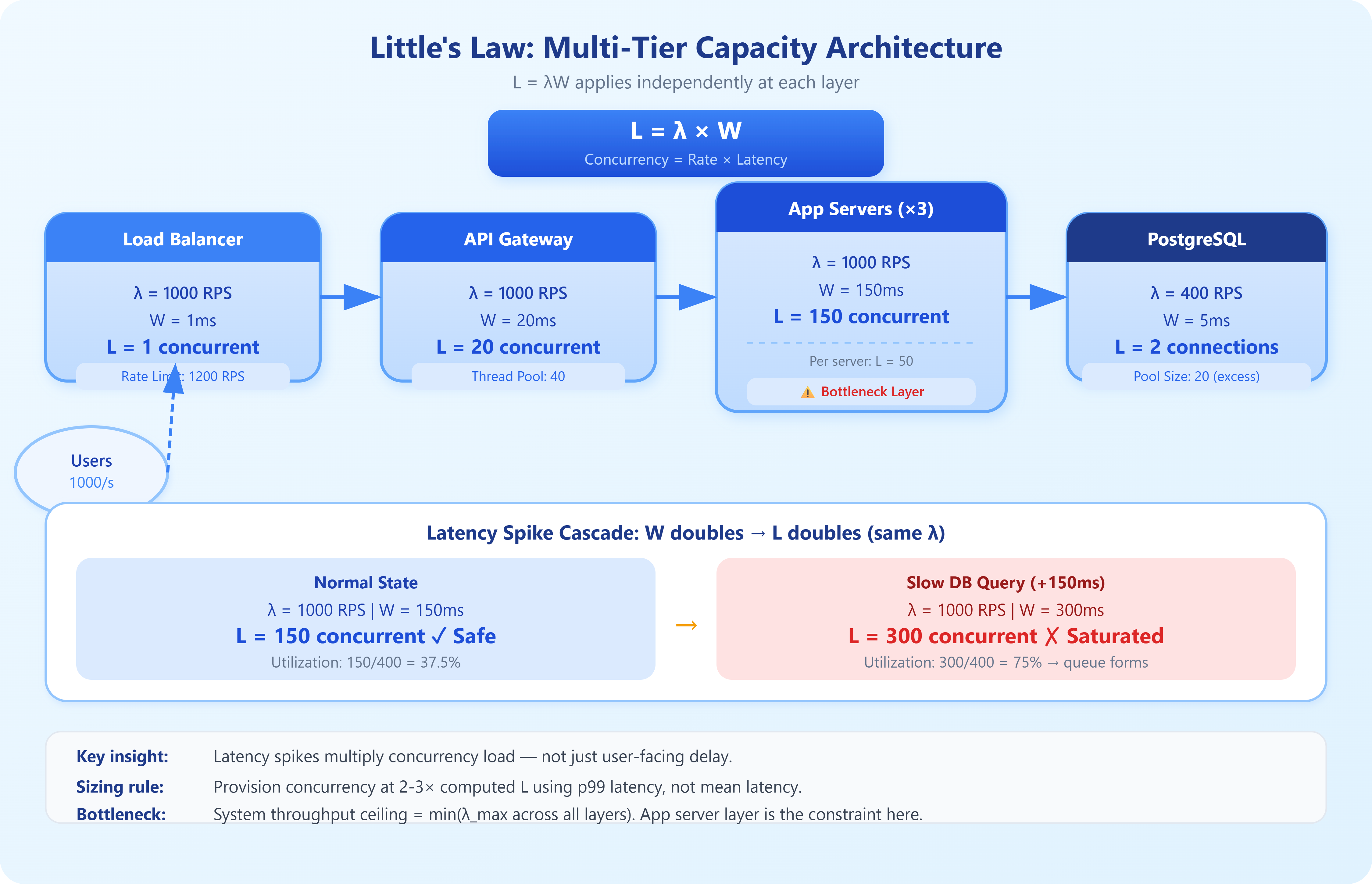
Segmenting by service tier: Apply Little’s Law independently to each layer. Your API gateway, application servers, database connection pool, and downstream service all have their own L, λ, and W. A bottleneck in any one layer creates backpressure upstream. The system’s actual throughput ceiling is the minimum across all layers — classic bottleneck analysis meets queueing theory.
Stability condition: Little’s Law only applies to stable queues where arrival rate doesn’t permanently exceed service rate (λ < μ, where μ is your service rate). When load exceeds capacity, queues grow without bound. This is why your 95th-percentile latency explodes suddenly at saturation — you’ve crossed the stability boundary.