
The probe
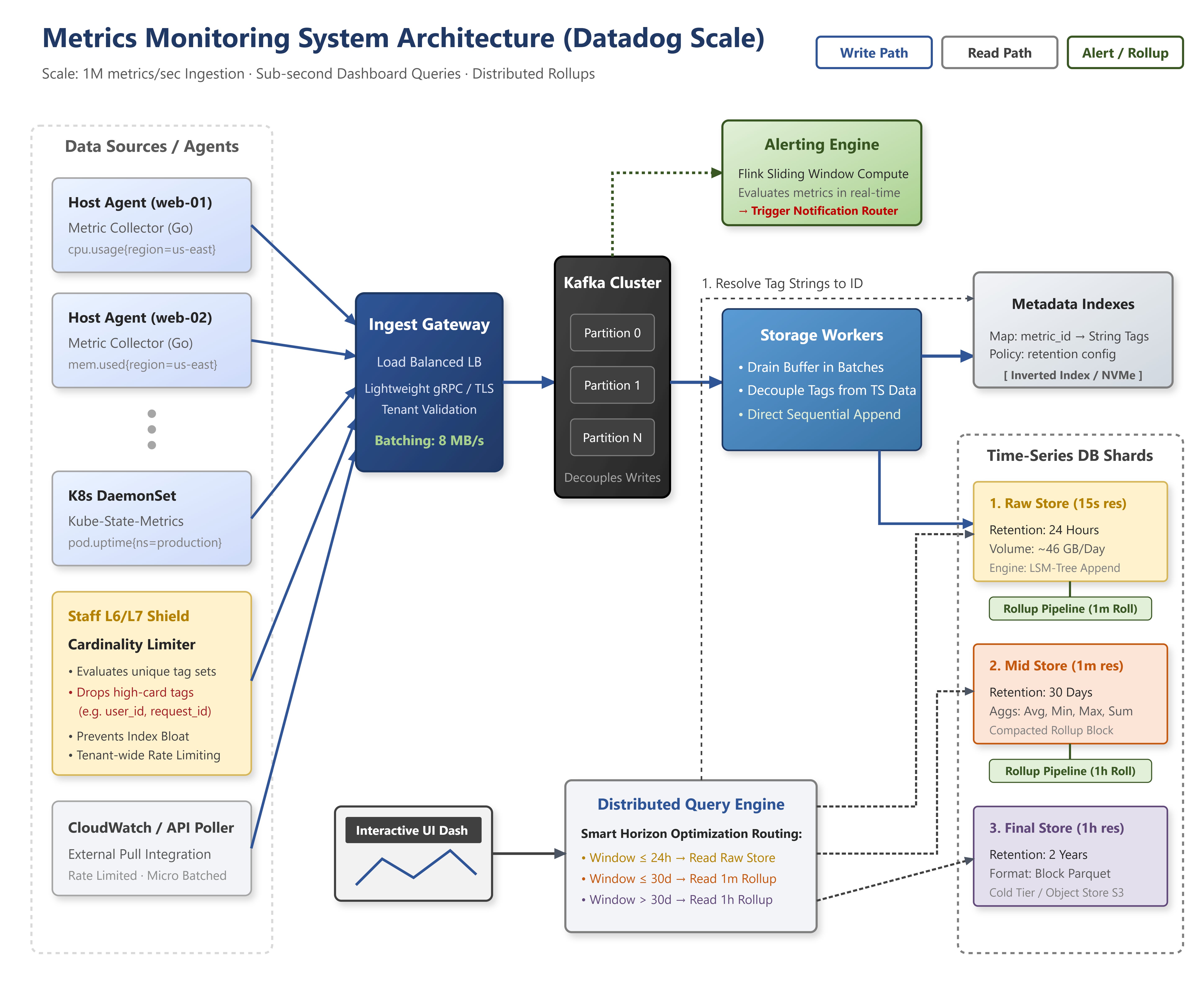
Time-series data at massive scale. The interesting problem is write throughput (millions of metrics per second from thousands of servers) vs query throughput (interactive dashboards needing sub-second response over months of data). These two requirements pull the architecture in opposite directions — you optimize writes by sequential append, you optimize range queries by pre-aggregation.
Step 1 — Clarify
- What types of data: metrics (numeric time-series), logs (text events), traces (distributed request spans)? Scope to metrics.
- Ingestion rate: 1M metrics/sec (single large deployment)
- Query SLO: dashboard queries over last 24h should return in < 2 seconds - Retention: 15-second resolution for 24h, 1-minute resolution for 30 days, 1-hour resolution for 2 years
- Alerting required? (Yes — threshold-based and anomaly-detection alerts)
Step 2 — Estimate
- 1M metrics/sec × 8 bytes/datapoint = 8 MB/sec write throughput
- At 15-second resolution: 1M × 4 datapoints/min × 60min × 24h = 5.8B datapoints/day - At 8 bytes/point: 46 GB/day raw. Over 30 days: 1.4 TB
- With rollup (15s → 1min → 1h): ~50GB/month per compression tier
Step 3 — Data Model
Time-series storage: Each metric is identified by a metric name + tag set (e.g., cpu.usage{host=web-01, region=us-east}). Stored as:
- Metric metadata: metric_id → {name, tags, retention_policy}
- Datapoints: (metric_id, timestamp) → value — ordered by timestamp, stored in a write-optimized time-series DB (InfluxDB, Prometheus TSDB, or custom LSM-tree)
Rollup tables: Three separate tables — raw (15s resolution), hourly (pre-aggregated to 1-minute), daily (pre-aggregated to 1-hour). Background jobs roll raw data up periodically, dropping the raw data after the retention window.
Preparing for a distributed systems interview?
→Download the free Interview Pack
→ Subscribe now to access source code repository - 200 + coding lessons
